43 excel line graph axis labels

How to rotate axis labels in chart in Excel? If you are using Microsoft Excel 2013, you can rotate the axis labels with following steps: 1. Go to the chart and right click its axis labels you will rotate, and select the Format Axis from the context menu. 2. How to wrap X axis labels in a chart in Excel? And you can do as follows: 1. Double click a label cell, and put the cursor at the place where you will break the label. 2. Add a hard return or carriages with pressing the Alt + Enter keys simultaneously. 3. Add hard returns to other label cells which you want the labels wrapped in the chart axis.

How to Add Axis Labels to a Chart in Excel | CustomGuide In the Chart Elements menu, click the Data Labels list arrow to change the position of the data labels. Display a Data Table. A data table is a table that contains the data and headings from your worksheet that comprises the chart data. Select the chart. Click the Chart Elements button. Click the Data Table check box.

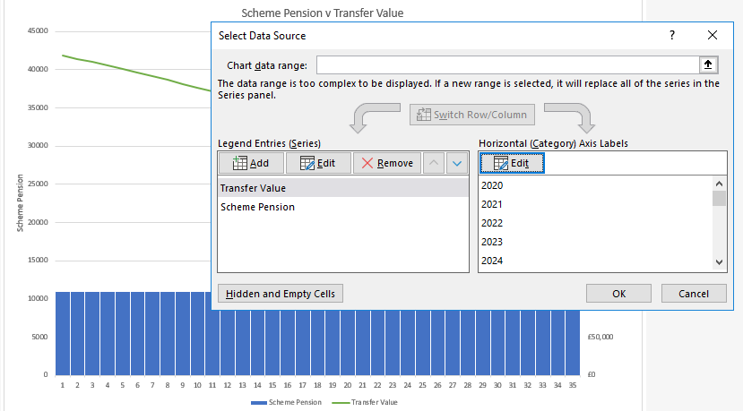
Excel line graph axis labels

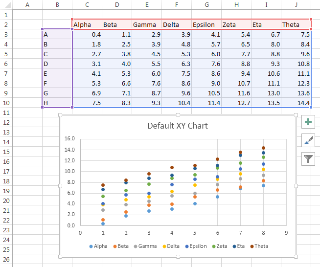
How to make a 3 Axis Graph using Excel? - GeeksforGeeks 29.03.2022 · To create a 3 axis graph follow the following steps: Step 1: Select table B3:E12.Then go to Insert Tab, and select the Scatter with Chart Lines and Marker Chart.. Step 2: A Line chart with a primary axis will be created. Step 3: The primary axis of the chart will be Temperature, the secondary axis will be Pressure and the third axis will be Volume. Change axis labels in a chart - Microsoft Support Right-click the category labels you want to change, and click Select Data. In the Horizontal (Category) Axis Labels box, click Edit. In the Axis label range box, enter the labels you want to use, separated by commas. For example, type Quarter 1,Quarter 2,Quarter 3,Quarter 4. Change the format of text and numbers in labels How to Add Axis Labels in Excel - Spreadsheeto If you would only like to add a title/label for one axis (horizontal or vertical), click the right arrow beside 'Axis Titles' and select which axis you would like to add a title/label. Editing the Axis Titles After adding the label, you would have to rename them yourself. There are two ways you can go about this: Manually retype the titles

Excel line graph axis labels. Two-Level Axis Labels (Microsoft Excel) Excel automatically recognizes that you have two rows being used for the X-axis labels, and formats the chart correctly. (See Figure 1.) Since the X-axis labels appear beneath the chart data, the order of the label rows is reversed—exactly as mentioned at the first of this tip. Figure 1. Two-level axis labels are created automatically by Excel. How to add Axis Labels (X & Y) in Excel & Google Sheets Adding Axis Labels Double Click on your Axis Select Charts & Axis Titles 3. Click on the Axis Title you want to Change (Horizontal or Vertical Axis) 4. Type in your Title Name Axis Labels Provide Clarity Once you change the title for both axes, the user will now better understand the graph. Add or remove data labels in a chart - support.microsoft.com On the Design tab, in the Chart Layouts group, click Add Chart Element, choose Data Labels, and then click None. Click a data label one time to select all data labels in a data series or two times to select just one data label that you want to delete, and then press DELETE. Right-click a data label, and then click Delete. How to Make Line Graphs in Excel | Smartsheet Step-by-Step Instructions to Build a Line Graph in Excel. Once you collect the data you want to chart, the first step is to enter it into Excel. The first column will be the time segments (hour, day, month, etc.), and the second will be the data collected (muffins sold, etc.). Highlight both columns of data and click Charts > Line > and make ...

How to Add Axis Titles in a Microsoft Excel Chart - How-To Geek 17 Dec 2021 — Add Axis Titles to a Chart in Excel ... Select your chart and then head to the Chart Design tab that displays. Click the Add Chart Element drop- ... How to Make a Line Graph in Microsoft Excel: 12 Steps 10.05.2022 · Enter your data. A line graph requires two axes in order to function. Enter your data into two columns. For ease of use, set your X-axis data (time) in the left column and your recorded observations in the right column. How to add Axis Labels (X & Y) in Excel & Google Sheets As a result, including labels to the X and Y axis is essential so that the user can see what is being measured in the graph. Excel offers several different charts and graphs to show your data. In this example, we are going to show a line graph … Excel tutorial: How to create a multi level axis To straighten out the labels, I need to restructure the data. First, I'll sort by region and then by activity. Next, I'll remove the extra, unneeded entries from the region column. The goal is to create an outline that reflects what you want to see in the axis labels. Now you can see we have a multi level category axis.

How to add a line in Excel graph: average line, benchmark, etc ... 12.09.2018 · This short tutorial will walk you through adding a line in Excel graph such as an average line, benchmark, trend line, etc. In the last week's tutorial, we were looking at how to make a line graph in Excel.In some situations, however, you may want to draw a horizontal line in another chart to compare the actual values with the target you wish to achieve. How To Add Axis Labels In Excel - BSUPERIOR Method 1- Add Axis Title by The Add Chart Element Option · Click on the chart area. · Go to the Design tab from the ribbon. · Click on the Add ... Dynamically Label Excel Chart Series Lines - My Online Training Hub Step 1: Duplicate the Series. The first trick here is that we have 2 series for each region; one for the line and one for the label, as you can see in the table below: Select columns B:J and insert a line chart (do not include column A). To modify the axis so the Year and Month labels are nested; right-click the chart > Select Data > Edit the ... Format Chart Axis in Excel - Axis Options However, In this blog, we will be working with Axis options, Tick marks, Labels, Number > Axis options> Axis options> Format Axis Pane. Axis Options: Axis Options There are multiple options So we will perform one by one. Changing Maximum and Minimum Bounds The first option is to adjust the maximum and minimum bounds for the axis.

microsoft excel - How to alter the horizontal axis labels on a bar graph to show a year long ...

3 Axis Graph Excel Method: Add a Third Y-Axis - EngineerExcel So he wanted to know if there was a way to create a 3 axis graph in Excel ... (the kind that look like plus signs), and changed the color of the line and marker to match the ... Add Data Labels To a Multiple Y-Axis Excel Chart. Axis labels were created by right-clicking on the series and selecting “Add Data Labels”. By default ...

spreadsheet - How to set different horizontal (category) labels for each different product in MS ...

How to Make a Bar Graph in Excel: 9 Steps (with Pictures) 02.05.2022 · Customize your graph's appearance. Once you decide on a graph format, you can use the "Design" section near the top of the Excel window to select a different template, change the colors used, or change the graph type entirely. The "Design" window only appears when your graph is selected. To select your graph, click it.

Excel Variance Charts: Making Awesome Actual vs Target Or Budget Graphs - How To ...

How to Insert Axis Labels In An Excel Chart | Excelchat We will go to Chart Design and select Add Chart Element Figure 6 - Insert axis labels in Excel In the drop-down menu, we will click on Axis Titles, and subsequently, select Primary vertical Figure 7 - Edit vertical axis labels in Excel Now, we can enter the name we want for the primary vertical axis label.

Excel Graph - horizontal axis labels not showing properly - Microsoft Community

Change the display of chart axes - Microsoft Support charts typically have two axes that are used to measure and categorize data: a vertical axis (also known as value axis or y axis), and a horizontal axis (also known as category axis or x axis). 3-d column, 3-d cone, or 3-d pyramid charts have a third axis, the depth axis (also known as series axis or z axis), so that data can be plotted along the …

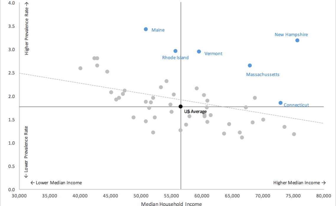
Excel Scatterplot with Custom Annotation - PolicyViz

How to Label Axes in Excel: 6 Steps (with Pictures) - wikiHow Select the graph. Click your graph to select it. 3 Click +. It's to the right of the top-right corner of the graph. This will open a drop-down menu. 4 Click the Axis Titles checkbox. It's near the top of the drop-down menu. Doing so checks the Axis Titles box and places text boxes next to the vertical axis and below the horizontal axis.

Intelligent Excel 2013 XY Charts - Peltier Tech Blog

Chart Axis - Use Text Instead of Numbers - Excel & Google Sheets Right click Graph Select Change Chart Type 3. Click on Combo 4. Select Graph next to XY Chart 5. Select Scatterplot 6. Select Scatterplot Series 7. Click Select Data 8. Select XY Chart Series 9. Click Edit 10. Select X Value with the 0 Values and click OK. Change Labels While clicking the new series, select the + Sign in the top right of the graph

Forum files

3 Types of Line Graph/Chart: + [Examples & Excel Tutorial] 20.04.2020 · Generate Line Graph. The next thing after formatting the data axis is to generate your line graph. To generate your line graph, highlight the cells containing your data. Navigate to the Insert tab on the menu, then click on Line to create a line chart for your data. Congratulations! You’ve successfully created a line graph in Excel.

Share :