44 data labels excel 2013
Excel 2013 Chart Labels don't appear properly - Microsoft Community 3. Both PC B and PC C couldn't see the chart data labels, either in the excel spreadsheet, or word or power point. Instead they saw Attachment B. 4. HOWEVER, today PC B forwarded the email to PC C and NOW PC C can see the data labels in the power point etc, AND the attachments from the older email from PC A are also visible in PC B. 5. Apply Custom Data Labels to Charted Points - Peltier Tech For data labels, the best tool by far is the XY chart label add in. I have Excel 2013 and have found that the Excel linked labels are not as reliable when the cells change as Rob Bovey's add in. Excel is complicated enough. We don't need to add complexity. Cheers,
Add or remove data labels in a chart - support.microsoft.com Right-click the data series or data label to display more data for, and then click Format Data Labels. Click Label Options and under Label Contains, select the Values From Cells checkbox. When the Data Label Range dialog box appears, go back to the spreadsheet and select the range for which you want the cell values to display as data labels.

Data labels excel 2013
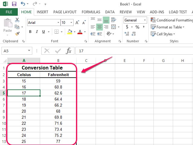
Excel Tips n Tricks -Tip 8 (Applying Chart Data Labels From a Range in ... Select the Column containing the text for the chart data and click "OK". Remember that the text should belong to the cell adjacent to the label data. Picture 7. 6. All done, just hit Enter or click "Ok" and you have your chart decorated with the text for data labels like this: Picture 8. Tip - Adding rich data labels to charts in Excel 2013 You can do this by adjusting the zoom control on the bottom right corner of Excel’s chrome. Then, select the value in the data label and hit the right-arrow key on your keyboard. The story behind the data in our example is that the temperature increased significantly on Wednesday and that appeared to help drive up business at the lemonade stand. Custom Data Labels with Colors and Symbols in Excel Charts - [How To] Step 4: Select the data in column C and hit Ctrl+1 to invoke format cell dialogue box. From left click custom and have your cursor in the type field and follow these steps: Press and Hold ALT key on the keyboard and on the Numpad hit 3 and 0 keys. Let go the ALT key and you will see that upward arrow is inserted.
Data labels excel 2013. How to Add Data Labels in Excel - Excelchat | Excelchat In Excel 2013 and the later versions we need to do the followings; Click anywhere in the chart area to display the Chart Elements button. Figure 5. Chart Elements Button. Click the Chart Elements button > Select the Data Labels, then click the Arrow to choose the data labels position. Figure 6. How to Add Data Labels in Excel 2013. formatting - How to format Microsoft Excel data labels without trailing ... To get this to work, I formatted the cell's of the data column 4 4 4 4 3.5 13.5, by either selecting the column and then right click and format cells or by right clicking on the chart and selecting format data labels.I formatted this with the regular expression $#K so that the data then shows as $4K $4K $4K $4K $4K $14K. The consequence is that the number is rounded to not include the decimal. Quick Tip: Excel 2013 offers flexible data labels - TechRepublic With the cursor inside that data label, right-click and choose Insert Data Label Field. In the next dialog, select. [Cell] Choose Cell. When Excel displays the source dialog, click the cell that ... Adding Data Labels to Your Chart - Excel ribbon tips To add data labels in Excel 2013 or Excel 2016, follow these steps: Activate the chart by clicking on it, if necessary. Make sure the Design tab of the ribbon is displayed. (This will appear when the chart is selected.) Click the Add Chart Element drop-down list. Select the Data Labels tool.
data labels in chart - excel 2013 | MrExcel Message Board Hi I have 3 data labels in column chart. I changed the shape of these labels to Oval Callout. if I select one of them to format, then they will be all selected as well. Which is good and understandable. But how can I move them all at same time. Now when I click on one of them then they will all... Adding rich data labels to charts in Excel 2013 - Microsoft Jun 21, 2013 · You can do this by adjusting the zoom control on the bottom right corner of Excel’s chrome. Then, select the value in the data label and hit the right-arrow key on your keyboard. The story behind the data in our example is that the temperature increased significantly on Wednesday and that appeared to help drive up business at the lemonade stand. Excel: Chart Labels in Excel 2013 - Excel Articles Excel Excel 2013 introduces a new feature where the chart labels can come from other cells on the worksheet. In the Figure below, formulas in column C build a label to identify the largest and second largest sales amount. ... Click the 3-Column chart icon in the Format Data Labels Task Pane. Click on Label Options. Checkmark Value From Cells ... Excel 2013 Tutorial Formatting Data Labels Microsoft Training Lesson 28 ... FREE Course! Click: about formatting data labels in Microsoft Excel at . A clip from Mastering Excel M...
Excel tutorial: How to use data labels Generally, the easiest way to show data labels to use the chart elements menu. When you check the box, you'll see data labels appear in the chart. If you have more than one data series, you can select a series first, then turn on data labels for that series only. You can even select a single bar, and show just one data label. How to Add Data Labels to your Excel Chart in Excel 2013 Watch this video to learn how to add data labels to your Excel 2013 chart. Data labels show the values next to the corresponding ch... Values From Cell: Missing Data Labels Option in Excel 2013? 8. May 27, 2015. #1. Ive inherited a Powerpoin with an embedded Excel chart and data sheet. The graph in Powerpoint shows several instances of a value [CellRange]. Im trying to figure out where its "trying" to pull its data from and I think because the data is not in a contiguous range its having trouble. A couple articles refer to formatting ... How to add or move data labels in Excel chart? - ExtendOffice To add or move data labels in a chart, you can do as below steps: In Excel 2013 or 2016. 1. Click the chart to show the Chart Elements button .. 2. Then click the Chart Elements, and check Data Labels, then you can click the arrow to choose an option about the data labels in the sub menu.See screenshot:
add labels to excel chart 218253.image0 - Top Label Maker
Creating a chart with dynamic labels - Microsoft Excel 2013 Excel 2013 365 2016. This tip shows how to create dynamically updated chart labels that depend on value or other cells. ... For all labels: on the Format Data Labels task pane, in the Label Options, in the Label Contains group, check Value From Cells and then choose cells:
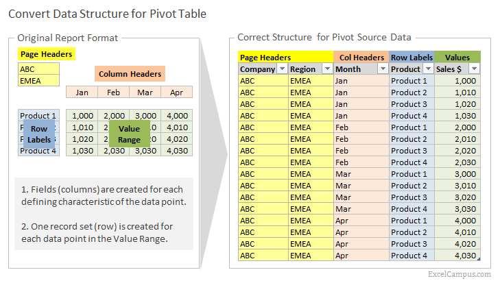
How to Setup Source Data for Pivot Tables - Unpivot in Excel
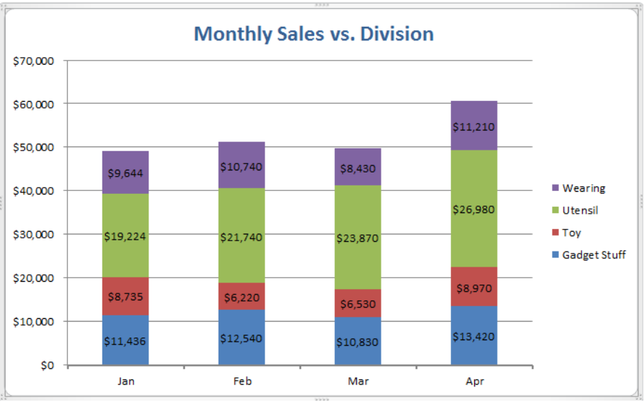
Custom Chart Labels Using Excel 2013 | MyExcelOnline View the Benchmark Chart using Excel 2013. DOWNLOAD EXCEL WORKBOOK. STEP 1: We added a % Variance column in our data and inserted symbols to show a negative and positive variance. ** You can see the tutorial of how this is done here **. STEP 2: In our graph we need to select the Sales chart and Right Click and choose Add Data Labels.
![How to Make a Pivot Table in Excel versions: 365, 2019, 2016 and 2013 [Includes Pivot Chart]](https://builtvisible.com/wp-content/uploads/2010/03/create-pivot-table.jpg)
How to Make a Pivot Table in Excel versions: 365, 2019, 2016 and 2013 [Includes Pivot Chart]
Values From Cell: Missing Data Labels Option in Excel 2013? When a chart created in 2013 using the "Values from Cell" data label option is opened with any earlier version of Excel, the data labels will show as " [CELLRANGE]". In the formula bar enter a formula that points to the cell that holds the desired label. This process can be tedious for larger charts with many labels.

Enable or Disable Excel Data Labels at the click of a button - How To - PakAccountants.com
How to Print Labels from Excel - Lifewire Select Mailings > Write & Insert Fields > Update Labels . Once you have the Excel spreadsheet and the Word document set up, you can merge the information and print your labels. Click Finish & Merge in the Finish group on the Mailings tab. Click Edit Individual Documents to preview how your printed labels will appear. Select All > OK .
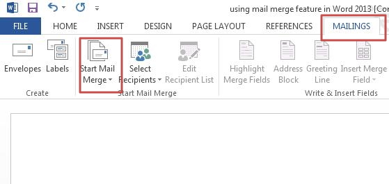
How to use Mail Merge feature in Word 2013 | Tutorials Tree: Learn Photoshop, Excel, Word ...
How to Customize Chart Elements in Excel 2013 - dummies To add data labels to your selected chart and position them, click the Chart Elements button next to the chart and then select the Data Labels check box before you select one of the following options on its continuation menu: Center to position the data labels in the middle of each data point. Inside End to position the data labels inside each ...

32 What Is A Data Label In Excel - Labels Design Ideas 2020
Change the format of data labels in a chart Tip: To switch from custom text back to the pre-built data labels, click Reset Label Text under Label Options. To format data labels, select your chart, and then in the Chart Design tab, click Add Chart Element > Data Labels > More Data Label Options. Click Label Options and under Label Contains, pick the options you want.
How to Add Data Labels in an Excel Chart in Excel 2010 - YouTube
How to add data labels from different column in an Excel chart? Please do as follows: 1. Right click the data series in the chart, and select Add Data Labels > Add Data Labels from the context menu to add data labels. 2. Right click the data series, and select Format Data Labels from the context menu. 3.

How to Create Multi-Category Chart in Excel - Excel Board
Format Data Labels in Excel- Instructions - TeachUcomp, Inc. To format data labels in Excel, choose the set of data labels to format. To do this, click the "Format" tab within the "Chart Tools" contextual tab in the Ribbon. Then select the data labels to format from the "Chart Elements" drop-down in the "Current Selection" button group. Then click the "Format Selection" button that ...

How to Add Data Labels in Excel - Excelchat | Excelchat
Custom Data Labels with Colors and Symbols in Excel Charts - [How To] Step 4: Select the data in column C and hit Ctrl+1 to invoke format cell dialogue box. From left click custom and have your cursor in the type field and follow these steps: Press and Hold ALT key on the keyboard and on the Numpad hit 3 and 0 keys. Let go the ALT key and you will see that upward arrow is inserted.

Multiple Series in One Excel Chart - Peltier Tech Blog
Tip - Adding rich data labels to charts in Excel 2013 You can do this by adjusting the zoom control on the bottom right corner of Excel’s chrome. Then, select the value in the data label and hit the right-arrow key on your keyboard. The story behind the data in our example is that the temperature increased significantly on Wednesday and that appeared to help drive up business at the lemonade stand.
Format Number Options for Chart Data Labels in Excel 2011 for Mac
Excel Tips n Tricks -Tip 8 (Applying Chart Data Labels From a Range in ... Select the Column containing the text for the chart data and click "OK". Remember that the text should belong to the cell adjacent to the label data. Picture 7. 6. All done, just hit Enter or click "Ok" and you have your chart decorated with the text for data labels like this: Picture 8.
How to Make an XY Graph on Excel | Techwalla.com
Excel Custom Chart Labels • My Online Training Hub
How to Add Data Labels in Excel - Excelchat | Excelchat
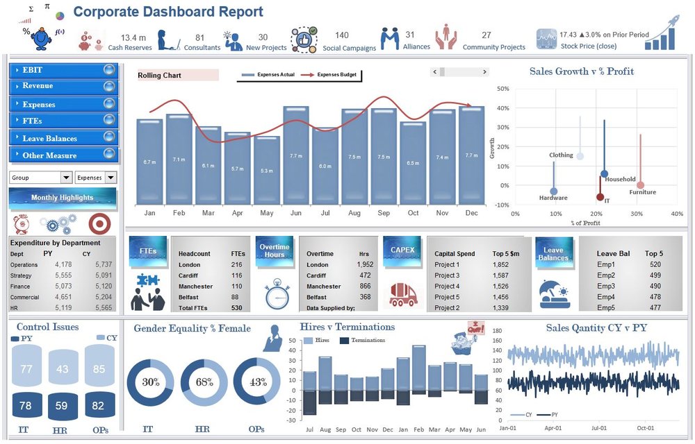
EBIT Excel Dashboard — Excel Dashboards VBA and more

r - Subgroup axes ggplot2 similar to Excel PivotChart - Stack Overflow
Post a Comment for "44 data labels excel 2013"